Ever notice that predictions almost always look better in aggregate? That is, summing a group of predictions seem to seems to result in an error lower than that of the individual predictions themselves.

Take a look at the following plot which shows this effect on the Boston housing dataset. On the left are predictions of median home price of towns near Boston (127 in all, taken from a randomly assigned test set) vs. to the actual median home price of the town. For the purpose of this post, each town was (randomly) assigned to one of 25 groups and predicted prices for each group were summed and compared sums of the actual prices as shown on the right.

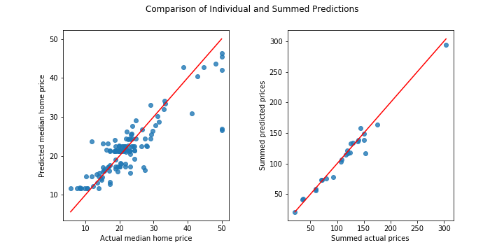
Notice how the errors in the aggregated plot are smaller (proportionally, not in terms of absolute error) than the predictions at the instance level. This phenomenon shows up often in regression and can be very useful for certain applications. It turns out that this effect can be explained with some basic properties of statistics.

Consider the familiar expression below relating relating the outputs of a machine learning model, $f(x)$, to a target variable, $y$,

\[y_{i}=f(x_{i})+\epsilon_{i}\]

The common sense interpretation of this equation is that the outputs of a model miss the target variable by some error, $\epsilon$. The underlying theory of some models actually make specific assumptions about these errors. Linear regression, for example, assumes the error terms are independent and identically distributed normal random variables with mean 0.

Let’s adopt this assumption, which will prove useful for our discussion here. Suppose $\epsilon_{i}\sim N(0,\sigma)$ and that we have a set of indices $J$ we want to sum our predictions over (e.g. one of the groups represented in the scatter plot above on the right). If we stick with the notation from the equation above we can work out a similar expression with a new error term

\[\sum_{i\in J}^{}{\epsilon_{i}}=\sum_{i\in J}^{}{y_{i}}-\sum_{i\in J}^{}{f(x_{i})}\]

which we will rewrite as $E_{J}=Y_{J}-P_{J}$ to simplify our discussion below.

This is where some basic algebraic properties of random variables and the normal distribution come into play. Because of the assumption that each $\epsilon_{i}$ is an i.i.d. normal random variable $E$ itself is also a normally distributed random variable with mean $0$ and standard deviation $\sigma\sqrt{n_{J}}$.

This is going to get a bit hand wavy, but the key observation here is that the mean of the summed target variable, $Y_{J}$, scales linearly with the number of indices in $J$, $n_{J}$. However the errors remain centered at 0 while their standard deviation scales according to $\sqrt{n_{J}}$ , providing explanation for the results in the plot above.

We can use the housing data to visualize this a bit more rigorously than the side by side comparison does above. By estimating $\sigma$ from the errors on the train set we can plot the errors for each group, $E_{J}$, against the 95% confidence interval of $N(0,\sigma\sqrt{n_{J}})$, i.e. the distribution we expect the errors to follow (note it is a 95% confidence interval so we expect some errors to fall outside the range).

Application

The data in this post was chosen mostly for convenience (from sklearn.datasets import load_boston) and the idea of wanting to know the sum of median house prices takes a stretch of the imagination. Nonetheless, this principle is useful for a variety of real world applications. One common situation where this is true is when we are interested in predictions at a higher level than the level which the data is collected. Another situation is when the feature set is richer at the lower level and aggregating the data up to the actual level of interest hides this information. This provides some justification for making the modeling decision to train a model at the lower level and “roll up” the predictions to the higher level.