When Philadelphia first went into self-quarantine last month, realizing that I was going to be working from home for the foreseeable future, I went to building a playlist that I could listen to for a “while” without getting bored of.

Such a playlist would need to be fairly large, but I didn’t want to spend too much time curating it so I put together the following rules to determine which songs should be included.

1. Add all albums released between 2000 and 2010 that had at least one song I listened to during that time period. This accumulated about 48 hours of music.
2. Each day open up Spotify and restart the playlist on shuffle, removing songs I don’t like as they are played.

After a few weeks my wife was surprised to see that I was still removing songs from the playlist and that there were yet songs which hadn’t been played. Since my “curation process” is probabilistic this prompted some interesting questions.

For example, without listening to the entire playlist, can I estimate

1. How many songs I’ve listened to so far?
2. How many songs are left that I’m going to remove?
3. When I’ve removed all songs from the playlist?

We’ll address each of these questions in turn, with some basic statistical principles that can be evaluated on a (scientific) calculator. I’ve tried to keep the math light throughout the main body of the post so as not to loose sight of the problem solving. For those interested, I’ve tried to capture the intuition behind the solutions in the appendix at the end.

Where are we?

Bagging, the generalization of Random Forests and which stands for “bootstrap aggregating”, is not a bad place to start when thinking about answering the first question above. In bagging, one samples with replacement from a given data set to create $m$ new data sets, trains a model on each of these new trainings sets and then aggregates the results.

While model training is not relevant here the process of sampling with replacement is. If you read the Wikipedia page on bagging you’ll come across the fact that each of the $m$ data sets are made up of approximately 63% unique examples. (The actual number is $1-1/e$, if you’re interested in the calculation see this stackexchange post). This calculation assumes that each of the $m$ samples has the same number of examples as the original data set, however in general the number of unique samples is

\[n\left(1 - \frac{1}{N}\right)^{n}\]

where $n$ is the number of samples and $N$ is the population size we are sampling from (number of examples in the original data set).

In my case, I don’t know the exact values of $n$ or $N$ but 800 and 960 are educated guesses. This gives us $\approx 347$ unique songs listened to, or said another way, out of the roughly 800 songs I’ve listened to so far, 453 are repeats.

How much longer till we get there?

Now that we have an idea of how much of the playlist I’ve listened to so far, let’s consider estimating how many songs remain in the playlist that I’m ultimately going to remove after they play - for convenience I’ll refer to these songs as bad going forward, with emphasis to avoid suggesting that my personal taste of music reflects any sort of objective quality.

A standard approach is to begin with a sample of the playlist. That is, let it play on shuffle and keep track of how many songs are played in total ($n$) and how many were bad ($s$).

While writing this post I did exactly that, listening to a total of 21 songs, 6 of which were bad.

Now that we have some data, $D=(n=21, s=6)$, and a parameter we would like to estimate, namely the proportion of bad songs in the playlist we have all of the main ingredients to calculate $P(p\vert D)$ using Bayes rule (supposing we don’t care to treat certain values of $p$ as more likely than others).

In particular the probability that $p=\tilde{p}$ for $\tilde{p}\in[0,1]$ works out to

\[P(p=\tilde{p}\vert n,s)=\frac{(n+1)!}{s!(n-s)!}\tilde{p}^{s}(1-\tilde{p})^{n-s}\]

from which we can obtain obtain the following posterior probability for $p$.

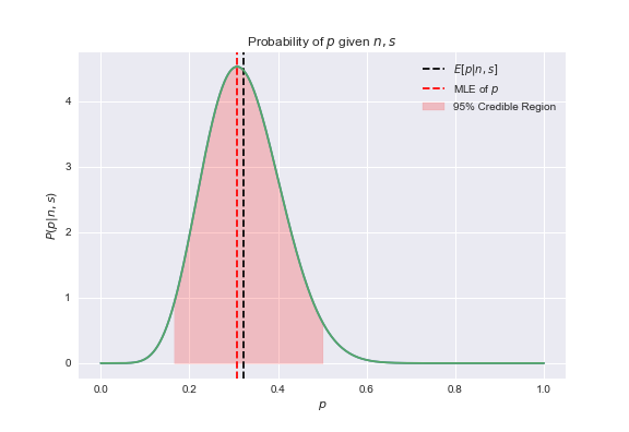
This shows the mode is centered at the maximum likelihood estimate of $6/21\approx .28$, but also suggests that values in the neighborhood of $[.2, .5]$ are also likely estimates for the proportion of bad songs in the playlist.

For details on deriving the equation above see here.

Are we there yet?

Finally “how will I know that all of the bad songs have been remove from the playlist?”

If we begin with sampling from the playlist once again we will find ourselves in a similar situation as before, however with two key differences.

First, let’s work with the principle that it would be premature to begin considering a criterion for testing whether all bad songs have been removed from the playlist before being reasonably sure that few, if any, bad songs remain in the first place. Operating under this principle, we wouldn’t want our criterion to be unduly “influenced” by large, irrelevant values of $p$.

In other words, unlike before, we want to explicitly treat some values as more likely than others, which is of course flirting with the idea of a prior.

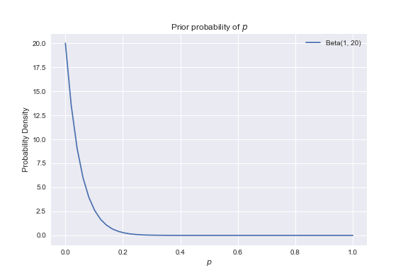
We’ll use the same underlying calculations to estimate $p$ as before, but this time placing a non-uniform prior on the probability of the value of $p$. In particular we’ll use $p\sim\text{Beta}(1, 20)$, which is a suitable choice for two reasons. First, the Beta distribution has a special relationship with the binomial distribution which makes simplifies calculating the posterior. Second, and more importantly, the prior easily expresses the belief that few, if any, bad songs remain in the playlist, as seen in the following plot.

The second important distinction to make from how we treated the sampling process above is that we are now considering a binomial trial where the number of successes (when a bad song plays) is always 0. This is because the moment a bad song plays it is immediately known that $p\not=0$. Thus the only value in our calculation that changes from one sample to the next is $n$, and we can do the calculations for $n=1\ldots$ before sampling.

Given $n$ trials with 0 songs found to be deleted we can calculate the mean posterior of $p$ as

\[E[P(p|n,\alpha=1,\beta=20)]=\frac{1}{21 + n}\]

The following plot shows how our estimate of $p$ is updated after $n$ consecutive “not bad” songs play. The expectation of the prior probability is included here, which gives us a nice visual of what John Kruschke means when he says Bayesian inference is about “reallocation of belief”. Keep in mind the axes here have completely different meanings than the plots above.

Of course, we can never know for sure that $p=0$ without listening to the entire playlist. However, the plot shows that with a little algebra we can easily develop a criteria that allows us to be reasonably sure that $p$ is very close to 0 without listening to anywhere near the entire playlist. For example if 80 songs play, without any one of them being bad we can be reasonably sure that $p<0.01$.

Lessons learned

Obviously this is a toy problem, but are there any useful take aways? I think so.

In my opinion, the main lesson to be learned here that having a familiarity with “variety” of well known problems can be immensely valuable when approaching something new if you can recognize which ones are relevant.

For example, while the calculations borrowed from bagging above are not perfectly suited to the actual problem we considered here it’s nevertheless a useful starting point. In bagging one takes $n$ samples with replacement $m$ times. However, here the setup is to take $n^{\prime}<n$ samples without replacement $m$ times. Moreover, because bad songs are being remove in real time $n$ is changing all the time. These are obviously different sampling procedures, where the latter is more difficult to solve. Nevertheless, as $m$ grows, our experiment will begin to look more like sampling with replacement. Thus, by identifying a similar, but simpler, problem we can quickly arrive at an approximation perhaps buying and serve as a sanity check while working on the more difficult problem.

For another example, consider the calculations we used to estimate the proportion of songs remaining in the playlist that I will remove. At first glance this is a straightforward application of Bayes theorem that doesn’t require any further context. Before simplifying terms, the expression is

\[P(p\vert n,s)=\frac{P(n,s\vert p)P(p)}{P(D)}\]

While the numerator is a simple maximum likelihood estimate calculation and a flat prior which are easy to calculate, the denominator requires an integral that is much more difficult.

\[P(D)=\int_{0}^{1}{q^{s}(1-q^{n-s}) \ \text{d}q}\]

In fact, this reminds us that often $P(D)$ cannot be calculated analytically. Fortunately the problem we are trying to solve here is the well-known Rule of Succession whose wiki page reminds us

\[\int_{0}^{1}{q^{s}(1-q^{n-s}) \ \text{d}q}=\frac{s!(n-s)!}{(n+1)!}\]

Of course, there’s always Wolfram Alpha for those, like myself, whose calculus skills are a bit rusty, but recognizing that this is well studied problem gives us access to a bit more context and might help point us to other useful resources.

Appendix

Resources

If the lesson learned here is to seek to familiarize oneself with foundations of data science and classic industry use cases, reading is one of the best ways to accomplish this goal. In fact this post inspired me to keep a running list of some of the resources I routinely visit to keep in touch with the industry at large here. Hopefully others may find this list useful.

Hints on deriving the expressions above

Counting the number of unique examples

The external resources I linked to above provide some helpful guidance on the identities and algebra required to derive the equations above. However these links don’t capture the intuition behind the derivations. I’ll try to provide some hints in that regard here.

For deriving the expected value of the unique number of samples it’s useful to remember that it’s sometimes easier to calculate the probability of an event not happening (known as the complement) than the probability that it does. This is almost always true if the complement can be expressed without using the word “or”. For example “The chance of $X$ and $Y$ and $Z$” instead of “The chance of $A$, or $B$, or $C$, or $A$ and $B$, …”. This is because if $X,Y,Z$ are all independent events the probability of the complement is can be calculated simply as the product of $P(X)P(Y)P(Z)$ without having to resort to combinations or permutations.

Thus if we want to calculate the probability that the example $x_{i}$ is in our samples $S$, it’s easier to work this out as

\[\begin{align*} P(x_{i}\text{ is in } S)&=1 - P(x_{i}\text{ is not in } S)\\ &=1-P(x_{i}\text{ was not first sample, and not second sample,} \ldots\text{and not $n^{th}$ sample})\\ &=1-\left(\frac{N-1}{N}\right)^n\\ &=1-\left(1-\frac{1}{N}\right)^n \end{align*}\]

Deriving the beta-binomial posterior

Let’s write out the complete beta-binomial model.

\[\begin{align*} &D=(n,s)&\text{ These are observed and fixed for all calculations.}\\ &P(p)=\frac{p^{\alpha-1}(1-p)^{\beta-1}}{B(\alpha,\beta)} &\text {This is our prior, $\alpha,\beta$ are fixed for all calculations.} \\ &P(D\vert p)={n\choose s} p^{s}(1-p)^{n-s} &\text{This is the binomial likelihood, and is determined by the experiment.}\\ &P(D)=\int_{0}^{1}{q^{n}(1-q)^{n-s}\ \text{d}q} &\text{The likelihood of the data, constant for all $p$} \end{align*}\]

Recalling the identity for $P(D)$ mentioned previously, we can plug these values into Bayes formula and simplify to get

\[P(p\vert D)=\frac{ {n\choose s}p^{\alpha+s-1}(1-p)^{\beta+n-s-1}}{B(s,n-s)B(\alpha,\beta)}\]

The algebra here is not terribly difficult. The challenge is understanding what we do and don’t need in the equation above.

Ignoring the terms which are fixed for all $p$ we have

\[P(p\vert D)\propto p^{\alpha+s-1}(1-p)^{\beta+n-s-1}\]

Why is this useful? Because PDFs represent relative probabilities. Since we have just demonstrated that the PDF above is proportional to the PDF of the beta distribution $\text{Beta}(\alpha^{\prime},\beta^{\prime})$, where $\alpha^{\prime}=\alpha+s$ and $\beta^{\prime}=\beta+n-s$, we can safely ignore the term ${n\choose s}(B(s,n-s)B(\alpha,\beta))^{-1}$ since it contributes nothing in terms of relative probability. This is why $P(D)$ is often referred to as simply a normalizing constant since it guarantees that $\int_{0}^{1}{P(p\vert D)\ \text{d}p}=1$ but contributes nothing else to the PDF.

Now that we’ve identified $\text{Beta}(\alpha^{\prime},\beta^{\prime})$ is the posterior distribution we can estimate $p$ from the mean of this distribution

\[\frac{\alpha+s}{\alpha+\beta+n-s}\]

which reduces to the our running estimate of $p$ as $n$ increases above when $s=0$.

This same reasoning is why we could safely ignore the uniform prior, $P(p)=c$, when we worked out the posterior probability of the proportion of bad songs remaining in the playlist.