Pete Alonso had a stellar 2019 season. One of his most significant achievements of this season was hitting 53 home, which set the record for number of home runs hit in a rookie season and helped him to win the Rookie of the Year award.

Given such a performance in the first year of Alonso’s major league career, it’s natural to ask what should we expect from him in his second season as the 2020 MLB season approaches. This question turns out to be an interesting question from a predictive viewpoint considering that it faces two distinct challenges.

Any player with a 53 home run season has “above average” talent. No struck of luck could be responsible for that kind of success. At the same time, a 53 home run season is pretty phenomenal and can reasonably be assumed to be an outlier. Thus it’s reasonable to expect the number of home runs hit by this player to “regress to the mean” in the following season. For Alonso the question is “what mean?” He’s clearly an above average player, but we only have one extraordinary season to gauge his talent by. This is our first challenge.

The second challenge is that, in general, an unprecedented number of home runs were hit across the league last year with 15 teams setting franchise records. This effect has been attributed in part to players adopting the “home run centric” play style of “launch angle” and in part to a “manufacturing inconsistency” that resulted in baseballs with less drag known as the juiced ball theory.

To summarize, predicting Alonso’s 2020 home run production is complicated by the following

1. 2019 was Pete’s first and only MLB season.
2. Its highly likely that his 2019 performance will be an outlier at the end of his major league career.
3. His 2019 campaign was likely influenced by a league-wide effect caused by an anomaly in the physical makeup of baseballs used throughout the 2019 season whose impact can’t be directly measured.

Bayesian stats to the rescue

To my eye, this problem is a perfect candidate for Bayesian inference. In particular for a technique known as partial pooling.

If you’re unfamiliar with partial pooling the pymc3 documentation has a clever example which estimates the batting average of a player with only 4 at bats and 0 hits. The tutorial shows that while the empirical batting average for this hypothetical player is 0 a partially pooled model estimates this player’s batting average much closer to the (data set’s) league average of 0.22-0.31. Partial pooling works by coupling global or population level parameters with individual or sub population parameters. In our case we should be able to use this technique to improve our estimates for Pete’s 2020 production from data on players with similar profiles to Alonso.

Additionally, we can include a parameter explicitly in our model to control for home runs hit due to the latent impact of juiced balls versus a player’s raw ability.

With pymc3 is a great library for fitting models like this in Python. In fact, with pymc3 we can build this model in under 50 lines of code - which include some generous whitespacing and comments on the choice of priors.

import warnings; warnings.filterwarnings("ignore")

import numpy as np
import pymc3 as pm
import theano as T

player_index = T.shared(df.player_id.values)
n_pa = T.shared(df.PA.values)
is_2019 = T.shared(df.year.eq(2019).astype(int).values)
n_players = len(encoder.categories_[0])


with pm.Model() as model:
    # Expect an average player to have around 10 home runs a season
    α = pm.Exponential('α', 1 / 10)
    
    # Interpretation of the beta-binomial distribution is α is the number of successes
    # and β is the number of failures. The interpretation here is α represents the
    # average number of home runs per 600 plate appearances.
    # See https://en.wikipedia.org/wiki/Conjugate_prior
    p = pm.Beta('p', α, 600 - α, shape=n_players)
    
    # We'll add this to the raw probability  estimated by the Beta distribution.
    # Since home run rates (per plate appearance) is typically much smaller than .1
    # we don't expect this prior to push the sampler into regions where p > 1 (even
    # though in threory p + juiced_ball could be larger than one).
    # The prior on the standard deviation is a heuristic making the conservative
    # assumption that the 2019 league total percent increase in home runs is less
    # than 1% not due to chance.
    juiced_ball = pm.HalfNormal('juiced_ball', ((6776 - 6105) / 6105) / 3)
    
    # Finally, represent the number of home runs hit by a player as a binomial
    # trial, conditioned on the number of plate appearances, the player's ability
    # and whether the 2019 juiced ball is in effect or not.
    homers = pm.Binomial('homers',
                         p=p[player_index] + is_2019 * juiced_ball,
                         n=n_pa,
                         observed=df.HR)

Pete’s 2020 campaign

So, how many home runs will Pete hit this season? As my high school statistics teacher used to teach us to say: “It depends.”

One of the things the answer depends on his how many opportunities Alonso has to hit a home run this season - he can’t knock one out of the park if he doesn’t step to the plate. If his season is shortened due to spending time in AAA or the IL we expect him to hit less home runs. By the same token, if the Mets make it to the post season he may have even more opportunities than last year.

Conditioning the predicted number of home runs on number of plate appearances allows us to control for this unknown and carries the additional benefits of being able to evaluate our predictions both in real time as the season progresses and after the season ends regardless of Alonso’s playing time.

These conditional predictions are shown in plot below on the left. For reference the actual number of home runs he had per plate appearance last year (calculated from MLBs Statcast data) are plotted alongside the 2020 predictions. The plot on the right provides additional context showing the predicted probabilities of Alonso’s 2020 HR season total given he has 693 PAs this year - the same as last. (Note of Alonso’s 693 PAs last year 5 are actually missing in the Statcast data I pulled. I’m uncertain which PAs exactly are missing but they don’t include any of the PAs home runs hit. Thus the plot is technically inaccurate, but for our purposes a good enough approximation.)

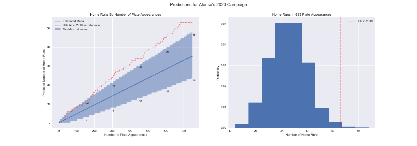
Another detail our answer depends on is whether the juiced ball returns this season - a topic which does not currently have a consensus with some sources claiming it may and others claiming it may not. To generate the predictions above I made the assumption that there is a 50/50 chance that it returns. However if we really wanted to hedge our bets we could condition the predictions on whether the baseballs in 2020 have “2019 drag” or “2012-2018 air resistance” (recall the data used for this analysis is 2012-2019).

To finish up here, if I were hard pressed to predict the number of home runs Pete Alonso hits in 2020 with numbers, and not plots, as the title of this post suggests, I’d use my P(ball is juiced)=1/2 assumption and condition my prediction on Alonso having somewhere between the nice round numbers of 675 and 715 PAs this season which gives Pete a 90% of hitting somewhere between 24 and 42 home runs.

Commentary

The statistical techniques demonstrated in this post really shine when applied to “small data” problems where a decision needs to be made.

Imagine being a GM interested in trading for Alonso. You would want to know just how much of an outlier his 2019 season was before deciding which players, cash or prospects are worth the trade. Of course the challenge is having only been able to watch him play for one season and if you wait for more data Alonso could be busy putting together a few more solid seasons, driving his trade value up. Whereas we would worry about a typical ML model overfitting in this situation, the hierarchical model described above uses domain knowledge and data from other MLB players to provide a robust prediction.

Another advantage of the probabilistic model in this situation is that it can provide more information than a single prediction alone to help guide the decision making process. You can imagine how your opinion on a trade might change if we forecasted Pete to hit 33-37 HRs vs. 24-42 HRs vs. 10-52 HRs.

I’ve intentionally kept the technical details in this post light. For more information I’ve written a number of posts on the topic, most of which link to even better external resources.