
Forecasting the final 100 or so games for all 30 MLB teams
One of my earliest posts on this blog was adapting Andrew Gelman’s “Stan Goes to the World Cup” model to rank MLB teams back in 2018. Over the years I’ve gotten quite a bit of mileage out of that model, using it for World Series projections that same year, for postseason projections in 2020 and then evaluating those projections after the 2020 season concluded. This year I’m using that same model to forecast wins for all 30 MLB teams over the remaining 100 or so games of the 2024 season.
A digression
We’ll get to the projections, but first a digression.
Each post on this blog has passed through a content filter. There aren’t explicit rules for what qualifies, but many a post has never seen the light on the other side of my GitHub.
It’s not that I’m trying to take a blog on a niche topic that gets a smallish amount of views each month too seriously, but each post needs to pass a simple “y, tho?” test. In general, a post that passes this test needs to
- be interesting
- offer something you can't find elsewhere online
- speak for itself, i.e. demonstrate that it works, a simple "take my word for it" won't make the cut
- have a clear point/conclusion
I also try to avoid redundancy - which means that given the number of MLB posts on this site, baseball topics face even more scrutiny.
So how did another baseball post on a model I’ve already written about three times make the cut?
A problem (interesting)
It all started with a conversation I was having with a colleague about the Phillies best-in-MLB record and their strength of schedule. This was a talking point that had been making its rounds in sports media at the time and went like this
The Phillies have not played a team with an above-.500 record since March 31… They’re on pace to be one of the best teams of all time. Can they actually keep that up?
It’s an interesting problem from a statistical perspective that can be framed in terms of sample size (it’s early in the season) and manifests itself as missing data (they haven’t played all 30 teams yet) and bias (they’ve played disproportionately subpar teams).
A big problem (a new take)
When I last wrote about this model I thought about it primarily in terms of latent variables and item response theory. But there was something about our conversation and thinking about how the model from my earlier posts would respond to the absence of a full season of data that gave me a new take on the intuition behind the model itself: in this context, I began to think of it as a big transitivity problem. Let me explain.
Recall that my first post on this subject was on learning to rank, so let’s start there, with the premise of a simple ranking model that assigns a scalar value, $a_{\text{team}}$, to each team. Under such a model we can express the problems of missing data and bias described above in terms of inequalities. Consider the following potential scenarios that could follow observing games between Colorado and Houston and Colorado and Miami.
| Scenario 1: Missing Data | Scenario 2: Bias |
|---|---|
| $$ \begin{align*} a_{\text{HOU}}<a_{\text{COL}}\\ a_{\text{COL}}<a_{\text{MIA}} \end{align*} $$ | $$ \begin{align*} a_{\text{COL}}<a_{\text{HOU}}\\ a_{\text{COL}}<a_{\text{MIA}} \end{align*} $$ |
In the first scenario, our ranking model does not necessarily need to observe games between the Astros and Marlins to infer, by transitivity, that $a_{\text{HOU}}<a_{\text{MIA}}$. So the issue of missing data shouldn’t be a problem - given enough data the nature of a ranking model can “fill in the gaps” itself.
On the other hand, it seems less clear how to infer the relationship between Houston and Miami in the second scenario where Colorado comes out on bottom in both matchups. Sure, Houston beat Colorado, but Miami did as well. It turns out however, that the original ranking model actually handles this quite well without any need for modification. To see how, we’ll need to turn to some more formal notation.
The model itself is Bayesian and its likelihood represents the number wins team $\text{team}{1}$ secures over team $\text{team}{2}$ in $n$ games as follows
\[\text{wins}_{\text{team}_{1}}\sim\text{Binomial}(n, p_{\text{team}_{1}})\]where
\[\begin{equation} p_{\text{team}_{1}}=\frac{\exp(a_{\text{team}_{1}})}{\exp(a_{\text{team}_{1}})+\exp(a_{\text{team}_{2}})} \label{eq:winprobability} \end{equation}\]Notice that it does not explicitly model rankings, rather it models wins and the rankings implicitly fall out of the math: the bigger $a_{\text{team}_{1}}$ relative to $a_{\text{team}_{2}}$ the better $\text{team}_{1}$’s win probability in the matchup.
Moreover, it doesn’t just predict wins, it learns to estimate win probabilities. This is key because it means that at the end of the day what comes out of $\eqref{eq:winprobability}$ needs to represent something interpretable as a probability. The effect is a sort of “regularization” of the values $a_{\text{team}}$. That is, because the rankings must live together in a latent space where their relative comparisons convert to probabilities, the model is prevented from overfitting to any one rank.
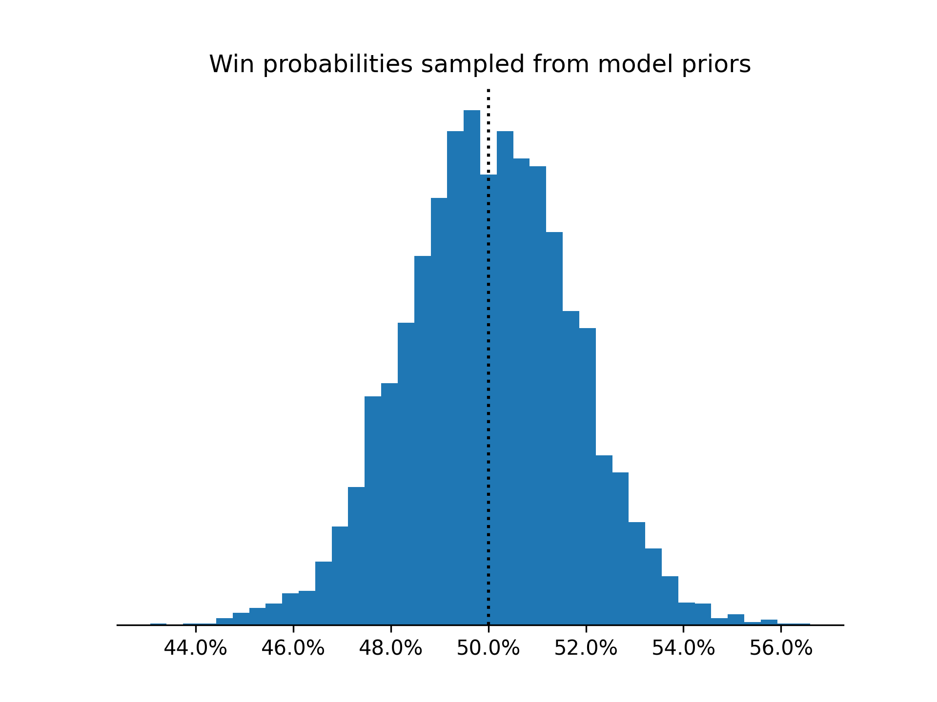
Since we are using a Bayesian model, we also use take advantage of using informative priors that center $p_{\text{team}}$ around .5 for any given pairs of teams and we partially pool the rankings $a_{\text{team}}$ across all seasons from 2015 to present.
Together, the likelihood, priors and partial pooling are what allows the model to gracefully handle the scenarios presented above. It’s worth noting however, that with enough data, it is the likelihood that really does the heavy lifting here. This is what Andrew Gelman has described as strain[ing] the gnat of the prior distribution while swallowing the camel that is the likelihood.
For completeness, you can expand to see full model details here
import pymc as pm
import pytensor.tensor as pt


def softmax(a):
    # reshaping for broadcasting
    a = pt.exp(a)
    sum_ = pt.sum(a, axis=1)[None, :].T
    return a / sum_

with pm.Model() as model:
    n_years = year_id.nunique()
    n_teams = home_team_id.nunique()
    year_id = pm.MutableData('year_id', year_id)
    home_team_id = pm.MutableData('home_team_id', home_team_id)
    away_team_id = pm.MutableData('away_team_id', away_team_id)
    N = pm.MutableData('N', N, dims='series')

    σ_a_μ = pm.Gamma('σ_a_μ', mu=np.log(5), sigma=np.log(5)/4)
    σ_a_σ = pm.Gamma('σ_a_σ', mu=np.log(5)/4, sigma=np.log(5)/8)
    σ_a = pm.Gamma('σ_a', mu=σ_a_μ, sigma=σ_a_σ)

    a_t = pm.Normal('a_t', mu=0, sigma=σ_a, shape=(n_years, n_teams))
    a_1, a_2 = a_t[year_id, home_team_id], a_t[year_id, away_team_id]
    a = pt.stack([a_1, a_2]).T

    p = pm.Deterministic('p', softmax(a))
    wins = pm.Multinomial(
        'wins',
        n=N,
        p=p,
        observed=game_outcomes,
        dims='series'
    )
Projections (let it speak for itself)
At this point, having shaken the dust off of an old model (and after updating some of the syntax to pymc 5.x), I had a new take on an old post that I found interesting. I was pretty happy with where all of this was going, but was it worth posting? Could it speak for itself? - the oft coup de grâce of a would-be-post.
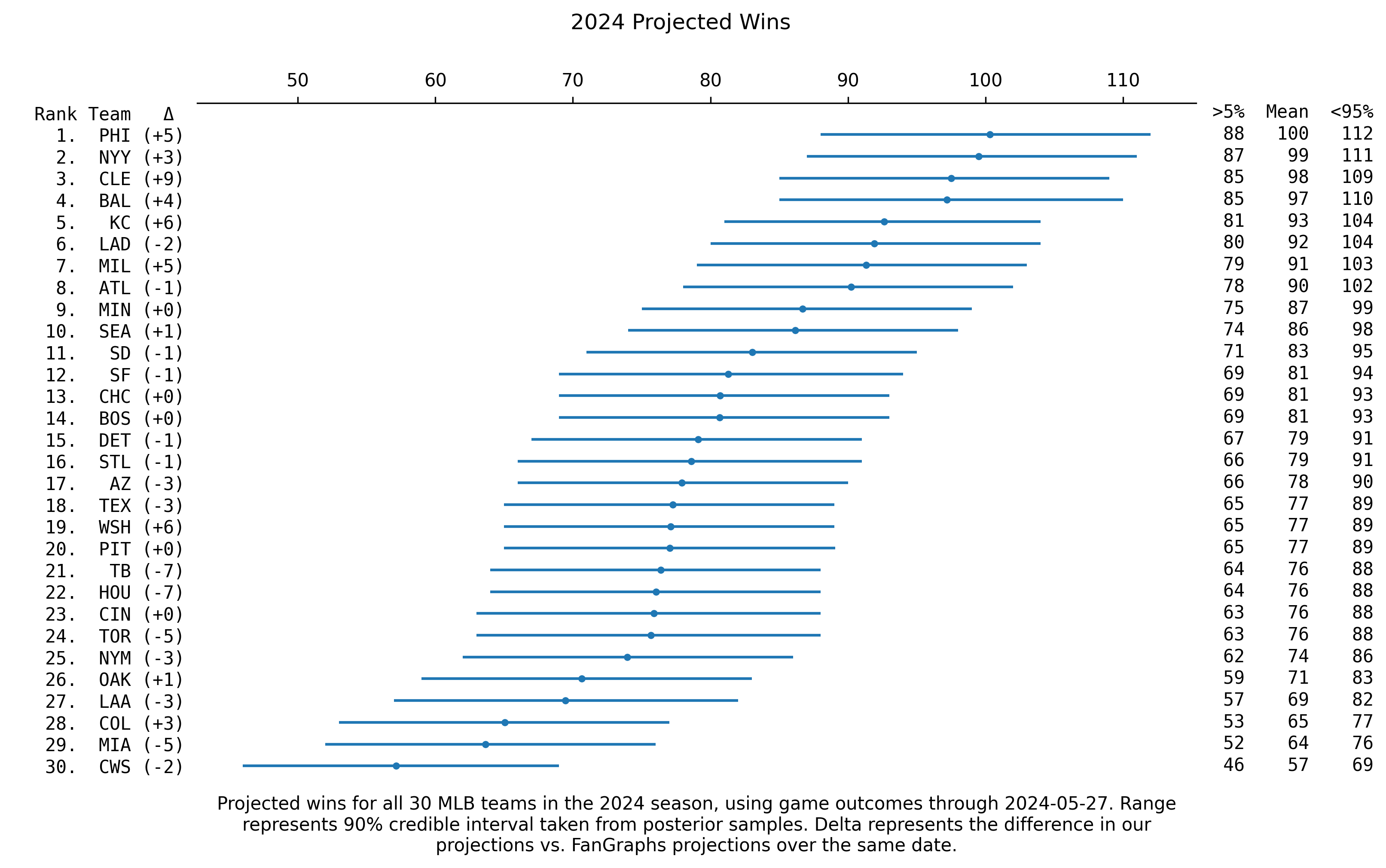
Eventually I decided it would be fun to put to the model to the test by forecasting the final 100 or so games for all 30 MLB teams. I really enjoyed putting the Pete Alonso home run predictions and 2020 post season predictions out there. It’s a great opportunity to demonstrate this method with a true forecast where the outcomes aren’t just a column in the data set that I have to pretend to ignore.
You can find the projections below. Each projection includes my forecast for the number of wins for the remainder of the season plus the team’s current wins. Because the model is probabilistic each projection includes a range of possible values corresponding to the 90% credible interval. Additionally, for comparison I’ve included the difference between my forecast and FanGraphs.
The point
So what’s the point? All of this underscores one of my favorite points to make about Bayesian Inference, which is that when you have the opportunity to map the model onto the way that world works you get so much more than just predictions.
Here we have this one model that accommodates asking questions about our data from different perspectives: which are the best teams? which are the worst? who will win the world series? How many wins will each team secure throughout the rest of the season?