This post is an adaptation of a talk I gave at Data Philly a couple of years ago.

Introduction

We’ve all seen it. That neon sign, hanging on some wall of some math department somewhere. Bayes’ theorem:

I would wager that Bayes’ Theorem is best known for calculating simple conditional probabilities, like the chance that a prize is behind door two, given a goat is behind door one. However, in my opinion, its best application is when it serves as the foundation of Bayesian Inference.

In practice, inference tends to be more interesting, because it accommodates a richer class of questions. Contrast the classic Monty Hall problem with the following: what is the chance that a prize is behind door two, given a goat is behind door one and the outcomes of past games?

This slight change in phrasing suddenly allows us to use data from previous games to consider questions like perhaps, every so often the game never had a prize, just to tilt the long-term odds in Monty’s favor.

In Bayesian Inference, (1) can be broken down into pieces that each play a specific role. In our discussion, I want to explore the possibilities of the left-hand side, which is known as the posterior distribution.¹

The posterior makes Bayesian Inference truly unique. It doesn’t give you just one predicted value. Instead, it produces a probability distribution over all possible values, with each probability directly informed by data.²

In my own experience, it took me quite a while to recognize the full potential of this property. For years I would reduce Bayesian models to a mean plus or minus a confidence interval,³ and, voilà, problem solved.

While this can be a reasonable approach at times, more often, it ends up leaving value on the table, or it would simply be more prudent to use techniques that are designed to produce point estimates in the first place if that’s what the job calls for.

In this post, I want to illustrate some of the unique opportunities the posterior distribution makes possible. To do so, we’ll work through an investing strategy described by Ed Thorp in an expository note published in the MAA, but with an added “Bayesian twist” to help drive our point home.

An investing strategy

As a physicist-turned-mathematician, Thorp turned his talents to Vegas, using an ingenious device invented with Claude Shannon, an original card-counting theory, and the Kelly criterion to beat the house. After overstaying his welcome in the city of lost wages, he returned to academia, only to change careers once again. And, once again, he found success in his new venture as a hedge fund manager by leaning on his past experiences - in particular, probability theory, applied mathematics, and a working knowledge of the Kelly criterion.⁴

It turns out that the Kelly criterion is central to our conversation. Developed by John Kelly at the legendary Bell Labs, the Kelly criterion seeks to maximize long-term wealth by repeatedly employing a “fixed-fractional” betting strategy that optimizes for geometric growth.

In the note referenced above, Thorp demonstrated that Kelly’s framework could be extended from a betting strategy for events with discrete outcomes to an investment strategy for events with continuous ones, like the S&P 500. This investment strategy will form the basis of our discussion.

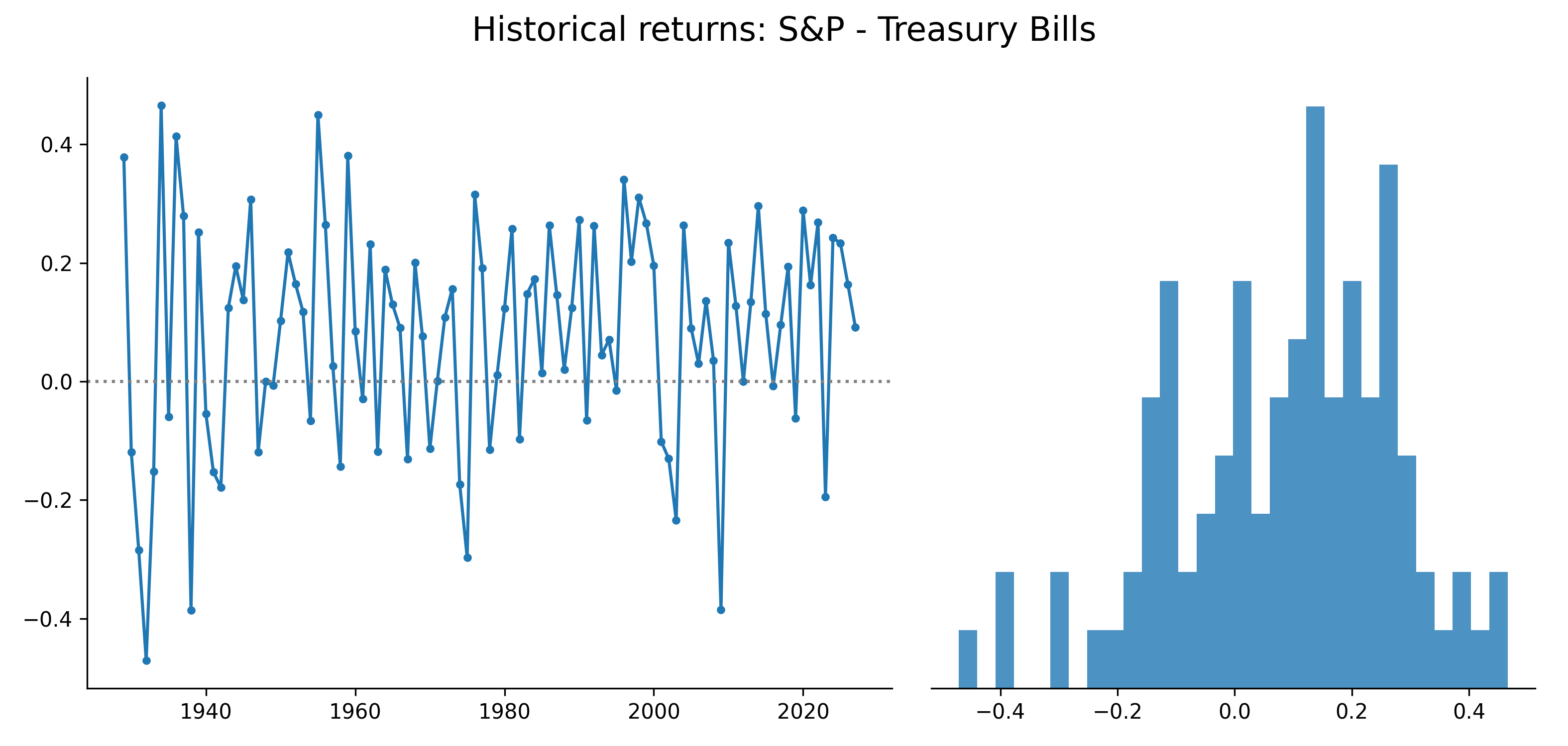
To get started, let’s begin by taking a look at those returns between 1928 and 2024.⁵

Following the Kelly criterion, Thorp too sought a fixed-fractional investment strategy, where an investor consistently reinvests their total wealth at a rate of $f$. The challenge is to avoid rates of $f$ that are too high and lead to eventual ruin (complete financial loss), or too low and diminish the potential of long-term gains.

Thorp showed that given an adequate probability model, let’s call it $p(s)$, which describes the (relative) probability of a return $s$, one should invest at the rate $f^{*}$ which solves the optimization problem

Let’s break down the integrand.

• If $\log(1 + fs)$ is the geometric growth rate of one’s wealth, when invested at a rate of $f$ for a return rate of $s$,
• then $p(s)\log(1+fs)$ is the probability-weighted geometric growth rate.
• Thus, integrating over $s$ gives us the expected geometric growth rate for our investment strategy $f$.

We can visualize this optimization problem by plotting each investment strategy, $f$, against the corresponding expected geometric growth rate.

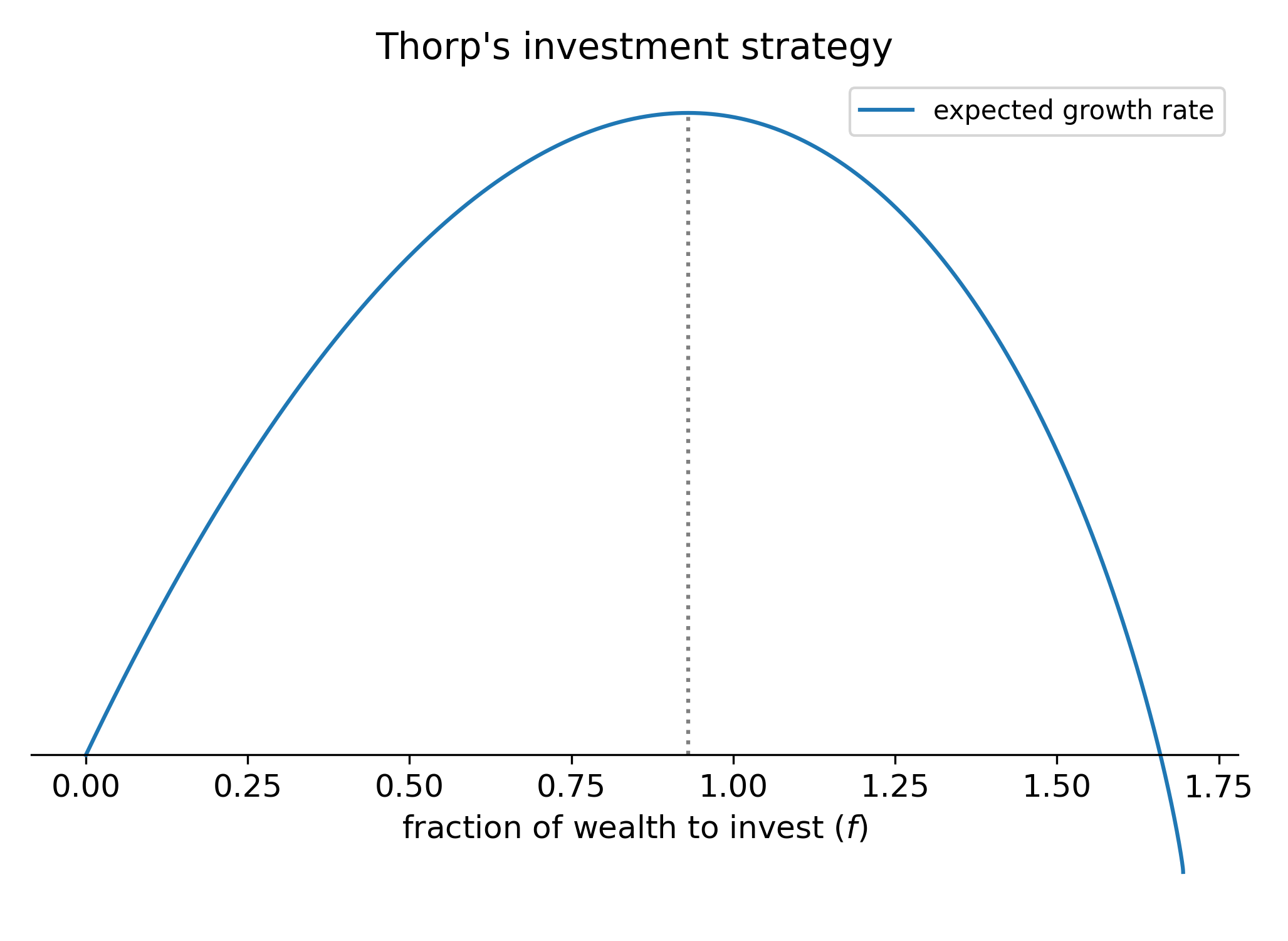
Thorp spent a lot of time carefully building the mathematical justification for several attributes about this problem that can be seen in the chart above:

• There is a unique, optimal investment rate $f^{*}$.
• Investing at rates beyond $f^{*}$ eventually leads to ruin (the “gambler’s dilemma”).
• The conditions under which the objective function will admit a meaningful solution $f^{*}$.
• How to find $f^{*}$ and how to avoid ruin.

Wading into those details is beyond the scope of this post, but it is crucial that we emphasize that those details exist. Going forward, it’s important to keep in mind that Thorp’s strategy, though perhaps somewhat intuitive when you think about it, is more than a heuristic - it is a method with theoretical grounding.

But, of course, all of this is true supposing that you have access to an adequate probability model, $p(s)$, in the first place.

Modeling the returns

Let’s use Thorp’s model as a starting point, with some choice modifications.

Keep in mind we’re not trying to one-up Thorp (who acknowledged his model as “somewhat artificially constructed” with limitations) or produce an oracle for S&P investments. Rather, we’re trying to develop an example that illustrates the unique properties of the posterior in Bayesian Inference.

Thorp took $p(s)$ to be a truncated normal distribution, and derived its mean and standard deviation empirically from the returns in his data set (the same as ours, but from the years 1926-1984) using maximum likelihood.

For our illustration, it’s sufficient to keep the normality assumption (which admittedly requires some hand-waving) but question the advisability of using a fixed pair $(\mu,\sigma)$, derived via maximum likelihood or otherwise.

Our main concern with choosing a fixed pair ($\mu, \sigma$) is that we risk bias due to our relatively small sample size. While this type of bias is always a concern when working on a model, it is especially so in our case where what may seem like small changes in these parameters can produce drastically different investment results.

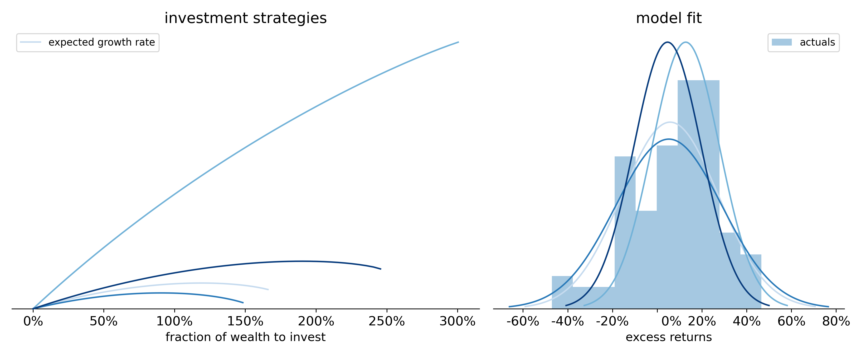
You can see this play out in the following chart. On the right, we show several values of $(\mu,\sigma)$ that plausibly fit our data. On the left are the corresponding investment strategies, which yield drastically different financial advice, ranging from investing less than 100% of one’s wealth to greater than 300% (implying heavy leverage).

Thus, the risk of producing an estimate that is slightly off could be the difference between massive over-investment (leading to ruin) or massive under-investment (leading to lost opportunity).

On the other hand, a Bayesian model produces a nice compromise. By treating $\mu$ and $\sigma$ as random variables while conditioning on past data, our estimates are informed by the data without being unduly committed to a single pair of model parameters.

Revisiting (2), the posterior expresses a probability distribution over $\mu$ and $\sigma$ conditional on past returns.

From posterior to posterior predictive

With the posterior on hand, we’re ready to tackle Thorp’s investing problem, but we’ll need to replace $p(\hat{s})$ with $p(\hat{s}\vert s)$ and adjust our notation, letting $\hat{s}$ and $s$ differentiate between arbitrary and historical returns to avoid ambiguity:

While it might look like a minor change, $p(\hat{s}\vert s)$ is a fundamental object in Bayesian Inference known as the posterior predictive distribution which positions us to introduce the posterior into the objective function.

Using the law of total probability, we can expand $p(\hat{s}\vert s)$ so that the expected growth rate is weighted over the posterior distribution in (5), becoming

This is our “Bayesian twist” on Thorp’s problem. By conditioning on the historical excess returns, we produce an objective function that is explicitly data-driven, without losing the theoretical support from Thorp’s work.

Now that our objective function is redefined in terms of the posterior, we simply need to solve it.

Putting it to use

Would it come as a surprise if I told you that equations, such as (6), that involve the posterior or posterior predictive range from difficult to impossible to calculate analytically? While this is true for all but certain special cases, there’s never been a better time to practice Bayesian Inference. That’s because numeric methods have never been faster or more reliable and are easier than ever to use with libraries like stan and pymc.

These numeric methods cleverly avoid the cumbersome integration required by expressions like $p(\hat{s}\vert s)$ altogether and instead draw samples from the posterior and posterior predictive:

How these methods work warrants its own discussion⁶, but note that this idea leans into the recognition that the posterior is a distribution.

With enough posterior samples, we can approximate the analytic solutions through simulation. For example, in our case, we can trade the integral in (5) for a weighted average over the posterior predictive samples $\hat{s}_{i}$,

From there, the right-hand side can be optimized in a number of ways.

With tools like pymc, the sampling procedure is rather straightforward.

1. First, we define the model parameters and data-generating process⁷
2. Then we generate samples that approximate draws from the posterior, $(\mu_{i},\sigma_{i})$
3. Each $(\mu_{i}, \sigma_{i})$ is used in turn to simulate a value from the posterior predictive, $\hat{s}_{i}$
4. Last, we simulate growth rates with $\log(1+f\hat{s}_{i})$

Steps 3 and 4 are sometimes called “forward sampling”, because each is determined from values in the prior step.

import numpy as np
import pymc as pm

with pm.Model() as model:
    # ↓↓↓ 1. define the model ↓↓↓
    μ = pm.Gamma('μ', mu=.04, sigma=.005)
    σ = pm.Gamma('σ', mu=.2, sigma=.05)
    likelihood = pm.Normal('likelihood', mu=μ, sigma=σ, observed=s)

    # ↓↓↓ 2. generate posterior samples: p(μ,σ ∣ s) ↓↓↓
    idata = pm.sample()

    # ↓↓↓ 3. generate posterior predictive samples  ↓↓↓
    # ↓↓↓    p(ŝ ∣ s) = p(ŝ ∣ μ, σ) × p(μ, σ ∣ s)   ↓↓↓
    pm.sample_posterior_predictive(idata, extend_inferencedata=True)

# ↓↓↓ 4. simulate the growth rate, for a given value `f` ↓↓↓
p_ŝ_given_s = idata.posterior_predictive.likelihood.values.ravel()

def expected_growth_rate(f):
    return -np.mean(np.log(1 + p_ŝ_given_s * f))

f_star = minimize(expected_growth_rate, ...)

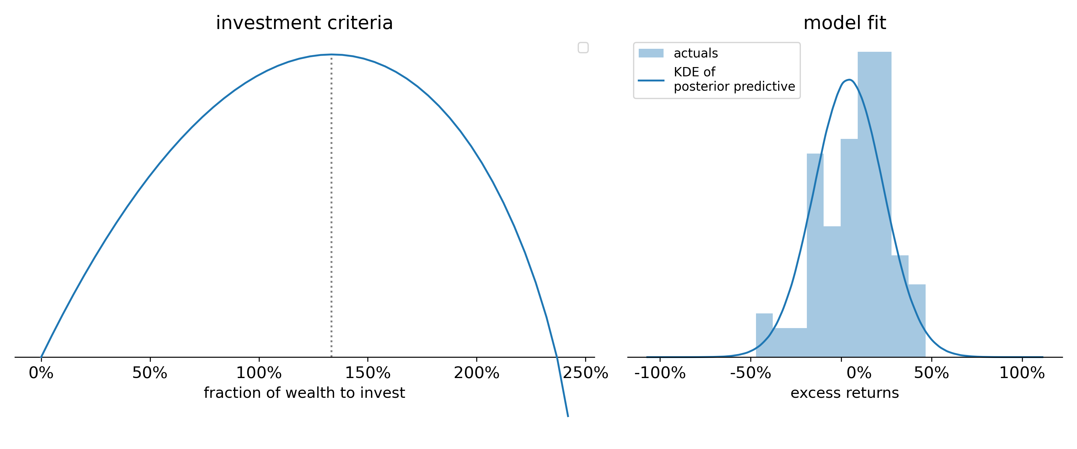
Applying this process to our data set results in the following model fit and investment criteria:⁸

Discussion

About a year ago I came across a quote from Allen Downey which summarizes our discussion well:

Bayesian methods don’t do the same things better; they do different things, which are better.

What is it that gives Bayesian methods these unique capabilities? Quoting Downey again, the posterior distribution is “exactly the information that makes Bayesian results more useful.”

However, I’ve taken this statement slightly out of context⁹, and perhaps it would be more fair to write

Bayesian methods don’t do the same things better; they do different things, which are [sometimes] better.

Conveniently, that single word, “sometimes”, is a reminder of this post’s primary goal: to provide a concrete illustration of the line between the sometimes Bayesian methods are better and the sometimes they are not.

If you’re making thousands of investment decisions a day, a week, or a month, a Bayesian model may be overkill. You might even be able to simplify Thorp’s strategy, using something like

where $s^{*}$ is a point estimate produced by a more traditional ML model. In fact, Google claimed to do something not too dissimilar to this in their real-time ad auctions.

And if you have googols of data, that’s probably fine. The variance on $s^{*}$ may be negligible, and the mean can provide a lot of mileage. But, if all you have are 106 data points, or you feel like you’re dealing with some other meaningful source of uncertainty, Bayesian methods like we’ve described here can provide a robust data-driven solution.

I hope that this recognition helps you resist the temptation to simply reduce the posterior to a mean $\pm$ some confidence interval and call it a day.¹⁰ Once this sinks in, and you’ve had an “I know kung fu” moment, you’ll begin to see that this post only scratches the surface.

In this example alone, it’s not hard to imagine future extensions of what we put together:

• What if we modeled the returns as a time series instead of a static distribution?
• What if we fit the model to a portfolio of funds, accounting for the covariance between them?
• How could we use Bayesian decision theory to learn a long-term strategy over time?
• $\ldots$

Footnotes